Data processing and file formats
| Site: | EUMETSAT Moodle |
| Course: | Short_course_07: The colour of the oceans |
| Book: | Data processing and file formats |
| Printed by: | Guest user |
| Date: | Wednesday, 24 April 2024, 4:15 PM |
Description
Within this book you will find two chapters. The first covers the processing that takes place to generate the data that is ultimately received by users of the CMDS. The second chapter goes in to the format of these data files, and the information that can be extracted from them.
1. Data formats and processing methodology: OLCI
Data levels
Within remote sensing and it's applications there are a series of levels that are used to define the amount of processing that has been performed to provide a given dataset:
-
Level 0 is the most raw data format available and refers to full resolution data, as it comes from the instrument, with some processing applied to remove artefacts from data communication between the satellite and the ground stations. It is unlikely you will work with this level of data, especially for more modern sensors, as this data lack information such as geo-referencing and time-referencing ancillary information.
-
Level 1 is further divided into A and B. Level 1A is the full resolution sensor data with time-referencing, ancillary information including radiometric and geometric calibration coefficients and georeferencing parameters computed and added to the file. Level 1B is the stage following the application of the parameters appended to the files at L1A (such as instrument calibration coefficients). This level also includes quality and classification flags.
-
e.g. for ocean colour this would be often referred to as the “top of atmosphere” radiance [mW.m-2.sr-1.nm-1].
-
-
Level 2 refers to derived geophysical variables. This will have required processing to remove the atmospheric component of the signal, as well as the application of algorithms to measurements to generate other products. This is the level at which many users will use the data, particularly if they are interested in event scale processes that require the highest time and space resolution available from the data stream.
- e.g. in the case of ocean colour, the core level 2 product is the water-leaving reflectance, whilst chlorophyll a is the commonly derived product. For OLCI these are available both at full resolution (300m pixel size) and reduced resolution (1km pixel size).
-
Levels 3 and 4 refer to binned and or merged/filled versions of the level 2 data for a given spatial or temporal resolution. The level 2 data from the CMDS feeds in to a further component of Copernicus (the Copernicus Marine Environmental Monitoring Service - CMEMS). This data can be useful for those wanting better spatial coverage, and those looking at marine processes that happen over longer time periods. In particular merged data can be used to generate long time series from multiple sensors, which is essential for climate studies.
The flow of data through these levels is illustrated in Figure 1.1 (taken from National Research Council, 2011). Obviously, as each layer builds on the processing that goes before it is of great importance to ensure that the early stages (such as calibration and atmospheric correction) are performed with a great deal of care and attention in order to ensure usable products for those wishing to implement algorithms at level 2 or beyond. The International Ocean Colour Coordinating Group (IOCCG) provide a wealth of information on the processing and uses of ocean colour data but of particular utility for information relating to data processing are IOCCG (1998, 2010, 2004).
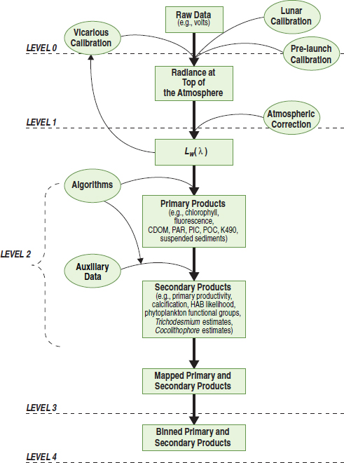
FIGURE 1.1 Ocean colour radiance is used to derive products directly or indirectly. Secondary products are based on the primary products and ancillary data. These products are then used to address scientific and societal questions. Some satellite missions apply the vicarious calibration when processing Level 2 data. (CDOM: Coloured Dissolved Organic Matter; PAR: Photosynthetically Available Radiance; PIC: Particulate Inorganic Carbon; POC: Particulate Organic Carbon; K490: diffuse attenuation coefficient at 490 nm; HAB: Harmful Algal Bloom).
Processing methodology
Atmospheric correction
The objective of ocean colour sensors is to retrieve the spectral distribution of upwelling radiance just above the sea surface, which is termed the water-leaving radiance (Lw). However, the sensors actually measure the Top Of Atmosphere (TOA) radiance (Lt) and so the contribution resulting from processes such as the atmosphere’s scattering and absorption needs to be accounted for – termed Atmospheric Correction (AC).
Lt(λ) = Lr(λ)+La(λ)+Lra(λ)+t(λ)Lwc(λ)+T(λ)Lg(λ)+t(λ)t0(λ)cos(θ0)Lwn(λ) (Eq. 1)
where Lr, La, Lra, Lwc, and Lg are radiance due to Rayleigh scattering, aerosol scattering, interaction between aerosols and molecules, white caps, and glint respectively. The terms t and t0 are diffuse transmittances of the atmosphere from the surface to the sensor and from the sun to the surface, T is the direct transmittance from surface to sensor, θ0 is the solar zenith angle and Lwn(λ) is the normalised water leaving radiance (see equation 4).
Over the first few decades of ocean-colour remote-sensing, various atmospheric correction algorithms were developed and implemented for a growing suite of sensors including OCTS, POLDER-1, SeaWiFS, MODIS-Terra, MODIS-Aqua, MERIS, GLI, POLDER-2, and VIIRS. It is of note that this computation requires ancillary information such as an estimate of the surface atmospheric pressure (and in some implementations, the surface wind speed is also used). The primary difference between these atmospheric correction algorithms is how the estimate of La(λ) + Lra(λ) in the visible wavelengths is derived from the estimate of La(λ) + Lra(λ) in the near infrared (NIR). Recently, there have been attempts to apply more complicated techniques to the problem of atmospheric correction, including spectral optimization (Shanmugam and Ahn 2007, Kuchink et al. 2009, Steinmetz et al. 2011) and neural networks (Schiller and Doerffer 1999, Brockmann et al. 2016), for particularly difficult areas (such as case 2 waters or regions of high glint). In these methods the atmospheric and oceanic parameters are retrieved simultaneously rather than sequentially.
Atmospheric correction for ocean colour data remains challenging (IOCCG, 2010) as only about 10% of the radiance measured by a satellite instrument in visible blue and green wavelengths originates from the water surface. This dictates that the sensors require a high signal to noise ratio (SNR), particularly for the ‘blue’ bands (~ 400 nm).
Once corrected for the influence of the atmosphere, the water-leaving radiance is converted to remote-sensing reflectance (Rrs in Eq. 1, where Es is the surface solar irradiance) or water-leaving reflectance (ρw Eq. 2). Then, there can be a further conversion to normalised water-leaving radiance (Lwn(λ) Eq. 3, where E0 is the average extra-atmospheric solar irradiance), which equates to a situation where that would exist if there were no atmosphere, and the sensor was at the nadir (directly above the point being viewed).
Rrs(λ) = Lw(λ)/Es(λ) (Eq. 2)
ρw(λ) = π Lw(λ)/Es(λ) (Eq. 3)
Lwn(λ) = Rrs(λ)E0(λ) (Eq. 4)
For OLCI, the ‘Baseline AC’ (BAC) algorithm is based on the algorithm developed for MERIS (Antoine and Morel, 1999), to ensure consistency between the two instruments' records. As it was designed for Case 1 waters, with a spectral signature dominated by phytoplankton pigments, then there is also a Bright Pixel AC (BPAC) integrated within it (Moore et al. 1999). The BPAC accounts for situations where the Near Infrared (NIR) water-leaving radiance is not negligible i.e., high scattering waters where there’s a high Chl and/or TSM concentration. The algorithm also provides aerosol optical depth (T865) and Ångström exponent (A865) that are calculated as part of the AC process, and indicate the AC’s success in estimating and subtracting the aerosol’s contribution; if the AC is working correctly then the atmospheric by-products shouldn’t show contamination from marine features.
Alternatively, for turbid Case 2 waters that are significantly influenced by CDOM and/or TSM, there is an artificial neural network algorithm (C2RCC); developed from work on algorithms for MERIS (Doerffer and Schiller, 2007).
Primary and secondary products
Once the surface reflectances and radiances have been calculated they can be used to estimate geophysical parameters through the application of specific bio-optical algorithms e.g. estimates of phytoplankton biomass through determining the Chlorophyll-a (Chl) concentration.
Again, taking OLCI as an example the algal pigment concentration is then estimated using the Ocean Colour for MERIS (OC4Me) algorithm developed by Morel et al. (2007). As with the atmospheric correction the best algorithm for a particular product of interest can depend upon the sensor used, the water type (such as case one or case two), the product itself (some algorithms are only designed to produce Chl products, while others estimate inherent optical properties) and even the atmospheric correction scheme used. Approaches range from simple band ratio algorithms to neural networks. Additionally there has recently been examples of improved product performance through the use of blended products (Jackson et al. 2017), where multiple algorithms are implemented and the final product is a weighted average, based on some other information such as a spectral classification (Moore et al. 2014).
File Names
A lot of thought goes into file naming conventions to provide useful information to the users without them even having to open the files. Consider an OLCI file for example for example:
S3A_OL_1_EFR____20160509T103945_20160509T104245_20160509T124907_0180_004_051_1979_MAR_O_NR_001.SEN3
In this example each underscore separates a field of information.
-
S3A is the mission (Sentinel 3A)
-
OL is the sensor (OLCI)
-
1 is the processing level
-
EFR is the Data type (“EFR___” = L1B TOA radiances at Full Resolution, "ERR___” = L1B TOA radiances at RR, “WFR___” = L2 FR water-leaving reflectance, ocean colour and atmospheric by-products, “WRR___” = L2 RR water-leaving reflectance, ocean colour and atmospheric by-products)
-
20160509T103945 is the date and time (follows the T) of the start of data acquisition
-
20160509T104245 is the date and time (follows the T) of the end of data acquisition
-
20160509T124907 is the date and time (follows the T) of the file creation
-
0180, 004, 051 and 1979 refer to duration, cycle number, relative orbit number and frame along track coordinate
-
MAR refers to the processing centre (MAR = Marine (EUMETSAT)
-
O means operational (a number of other possibilities include F for reference, D for development and R for reprocessing)
-
NR means “Near Real time” processing (the most rapidly available data released; other possibilities include NT - non time critical, which includes the most up to date meteorological data used for processing).
-
001 is the baseline collection
-
Finally .SEN3 is the filename extension (which data viewing programs etc may use for opening the file correctly).
File types
The file types listed below are the most common storage architecture for all sentinel-3 products, irrespective of sensor. While the discussion below refers to an ocean colour perspective, the information remains valid for both SLSTR and Altimetry domains.
NetCDF (Network Common Data Format)
These are self describing files that are commonly used for array-oriented scientific data. This is probably the most common file type you will come across while working with ocean color data.
HDF (Hierarchical Data Format)
This includes a set of file formats (e.g HDF4, HDF5) designed to store and organize large amounts of data. NetCDF users can create HDF5 files with benefits not available with the netCDF format, such as much larger files and multiple unlimited dimensions.
xml (Extensible Markup Language)
These files use a markup language that allows both human and machine readability of document encoding for textual data. Although xml was designed for use with documents, the language is widely used for the representation of data structures. You will find that folders of OLCI data can contain an xml file that allows all the various products, flags and metadata to be loaded into a program such as SNAP in a single operation.
2. Data formats and processing methodology: SLSTR
Data Levels
Within remote sensing of sea-surface temperature there are a series of levels that are used to define the amount of processing that has been performed to provide a given dataset:
-
Level 0: This step processes raw data contained in instruments source packets Level 0 products are internal products, and are not disseminated to users.
-
Level 1: This step processes the Level 0 data to geo-located radiometric measurements for each SLSTR channel/view. SLSTR Level 1 processing is divided into two main steps. Instrument grid processing (Level 1A) and image grid processing (Level 1B). The Level-1 product provides radiances and brightness temperatures for each pixel in a regular image grid, each view and each SLSTR channel, plus annotations data associated with SLSTR pixels.
-
Level 2: This step processes the Level 1 data to geophysical data (e.g. sea surface temperature, land surface temperature). It, again consists of two stages. In the first stage, SST processing to generate five single-algorithm SST products using various methods. These are provided in the Level 2 WCT product, which is not typically distributed. This is followed by a processing module, which generates a Group for High Resolution Sea Surface Temperature (GHRSST) compliant product, referred to as a Level 2 WST product, which is distributed.
Processing Methodology
SLSTR Level 1 processing is divided into two main steps (figure 2.1):
- Instrument grid processing
- Image grid processing
The instrument grid processing has five sub-steps (figure 2.1, left hand column). First the source packets from the instrument are processed. Next the data is calibrated: For the IR channels this involves calculating the calibration offset and slope that describes the linear relationship between numerical counts and radiance; for the VIS/NIR/SWIR channels, the calibration is based on a diffuse calibration (VISCAL) target of accurately known reflectance which is illuminated by the sun over a short segment of the orbit to enable a linear calibration relationship between the measured signal in each channel and the surface reflectance to be determined. Finally, the time and geolocation are calculated for each pixel.
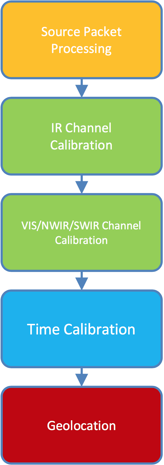
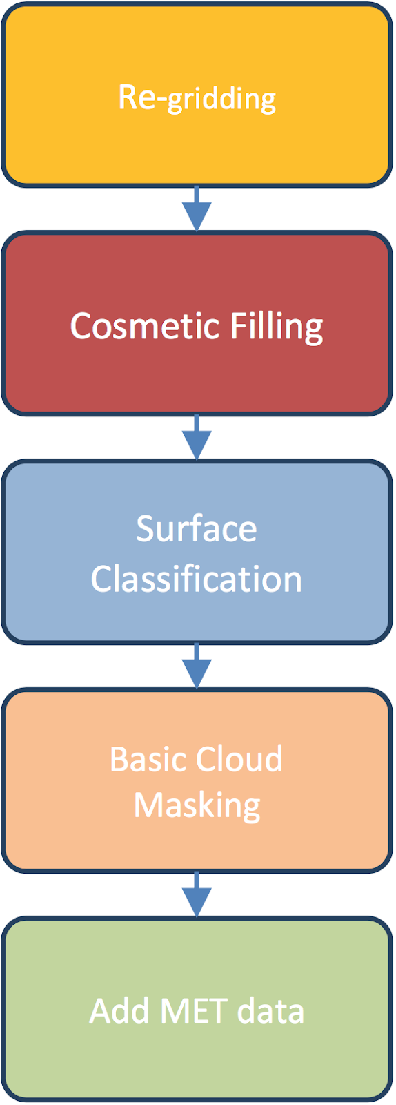
Figure 2.1; Level 1 processing stages for instrument grid processing (level 1A, left column) and image grid processing (level 1B, right column).
The image grid processing re-grids the SLSTR measurements onto the nominal raster image, and tests each pixel for cloud. It also contains five sub-steps (figure 2.1, right hand column).
In the re-gridding, the across and along track indices are calculated for each instrument pixel on either a 1 km raster image grid for the thermal IR channels or a 0.5 km grid for the visible, NIR and SWIR channels. The re-gridding is done by nearest neighbour resampling. Missing image pixels are then cosmetically filled.
The data is strictly speaking not cosmetic, i.e. it is not made up, it is simply that an instrument pixel might be used more than once. Instrument pixels that are not used in generating the image pixels are included in the orphan pixels’ containers. Surface Classification and the Basic Cloud Masking are then applied to each image pixel. Finally, the ECMWF meteorological fields are added on a sub-grid referred to as the tie-point grid.
SLSTR Level-2 marine processing includes two primary steps (figure 2.2):
- SST processing to generate five single-algorithm SST products using the method described in Section 3.5. These are provided in the Level 2 WCT product. The SSTs included are:
- 1 km N2 SST
- Nadir single view using channels S8 and S9, i.e. 10.85 and 12 μm
- 1 km N3 SST
- Nadir single view and all thermal channels (N2 plus S7, i.e. 3.7 μm)
- 1 km N3R SST
- Like N3 but using the property of "aerosol robustness" and its associated method described in [RD-5]
- 1 km D2 SST
- Like N2, except that BTs in both the oblique and nadir views are used
- 1 km D3 SST
- Like N3, except that both views are used.
- The L2P processing module, which generates a Group for High Resolution Sea Surface Temperature (GHRSST) compliant product. The L2P product contains only the best available SST for each pixel according to a set of rules define in the SLSTR Level 2 SST ATBD. In an extra step compared to the WCT product, the WST SSTs are atmospherically smoothed to reduce noise introduced in the retrieval process. Further details of the smoothing can be found in the SLSTR Level 2 SST ATBD. The L2P format data file is provided in the Level 2 WST product.
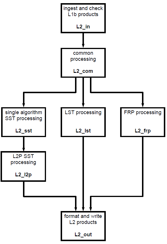
Figure 2.2; Level 2 processing stages for SLSTR.
The following products are generated at the levels described above;
Level 1 RBT
This product provides radiances and brightness temperatures for each pixel, view and channel.
Level 2 WCT (only available to Cal/Val users via S3VT)
This product provides sea surface temperature for all offered retrieval algorithms.
Level 2 WST
This product provides the best SST at each SLSTR location in GHRSST L2P format.
File Names
The file naming is based on a sequence of fields:
MMM_SS_L_TTTTTT_YYYYMMDDTHHMMSS_YYYYMMDDTHHMMSS_YYYYMMDDTHHMMSS_<instanceID><class_ID>.<extension>
Where;
-
MMM – Mission id, e.g. S3A
-
SS - Instrument e.g. SL is for SLSTR
-
L - Processing level, e.g. 1 for L1 and 2 for L2
-
TTTTT - Data Type ID, e.g.
-
“RBT___” = TOA radiances and brightness temperatures
-
“WCT___” = Retrieved SST for all algorithms
-
“WST___” = Best SST in GHRSST L2P format
-
-
YYYYMMDDTHHMMSS - 15 character Data Start time, then Data Stop time then Creation Date
-
<instance id > - 17 characters e.g. 0180_004_051_1979 is duration, cycle number, relative orbit number and frame along track coordinate GGG – Product Generating Centre e.g., EUM = EUMETSAT and SVL = Svalbard Satellite Core Ground Station
-
<class ID> - 8 characters to indicate the processing system e.g., O_NR_001 is the software platform (O for operational, F for reference, D for development and R for reprocessing), processing workflow (NR for Near Real Time, ST for Short Time Critical and NT for Non Time Critical) and 3 letters/digits indicating the baseline collection.
-
<extension> - Filename extension, SEN3
Which for Sentinel-3 SLSTR data would be, for example:
S3A_SL_1_RBT____20160509T103945_20160509T104245_20160509T124907_0180_004_051_1979_SVL_O_NR_001.SEN3
File types
Please see the ocean colour section.
3. Data formats and processing methodology: SRAL
Data levels
Within altimetry remote sensing there are a series of levels that are used to define the amount of processing that has been performed to provide a given dataset:
-
Level-0 is the raw telemetered data.
-
Level-1B is the Level-0 data corrected for instrumental and geometrical effects. The main function of the Level-1 processing chain is to calculate the tracker range, the sigma0 scaling factor and the Level-1 waveforms, applying instrumental corrections to all of them.The Level-1 processing chain outputs three types of products: Level-1A , Level-1B-s and Level-1B products.
-
Level-2 is the Level-1 data corrected for geophysical effects. The first function of the Level-2 processing chain is to apply different retracking algorithms to the Level-1 waveforms to calculate the final altimeter range, backscatter coefficient, wind speed over ocean and SWH. There are different types of re-tracking algorithms according to the type of waveforms re-tracked (ocean, ice, sea-ice).
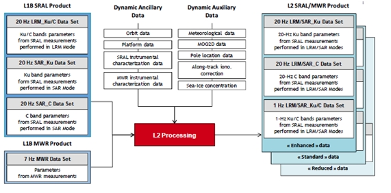
Figure 3.1; Level 2 processing stages for altimetry.
Processing Methodology
Level 0
The Level-0 product is an output from Level-0 processing and is an internal product only. The satellite sends all data measured to the ground stations in the form of Instrument Source Packets (ISP). The data in ISPs are categorised and packaged according to their type:
- TM_ACQ: telemetry packets generated during acquisition mode
- TM_CAL1: telemetry packets generated during CAL1 calibration mode
- TM_CAL2: telemetry packets generated during CAL2 calibration mode
- TM_ECHO_LRM: telemetry packets generated during LRM tracking mode
- TM_ECHO_SAR: telemetry packets generated during SAR tracking mode.
Level 1
The Level-1 calibration chain computes all calibration corrections. One part of these calibration corrections is characterised on the ground and one part is measured in flight. There are three types of calibrations:
- calibration due to internal calibration of the instrument (CAL1)
- calibration due to the gain profile range window (CAL2)
- calibration due to the calibration of the Automatic Gain Control (AGC) correction tables.
These calibration corrections are applied in the Level-1 measurement chains. There are two types of Level-1 processing measurement chains: one to process LRM and SAR-C band data and another to process SAR-Ku band data.
The main processing steps of the LRM and SAR-C Level-1 measurement chains are:
- Determine surface type.
- Correct tracker ranges for USO frequency drift.
- Compute internal path correction.
- Correct the AGC for instrumental errors.
- Compute Sigma0 scaling factor.
- Compute Doppler correction.
- Correct waveforms by CAL2.
The main processing steps of the SAR-Ku Level-1 measurement chain are:
- Determine surface type.
- Correct tracker ranges for USO frequency drift.
- Compute internal path correction.
- Correct the AGC for instrumental errors.
- Correct waveforms by CAL1 and CAL2.
- Compute surface locations.
- Apply Doppler correction.
- Apply slant range correction.
- Align the waveforms.
- Perform the Doppler beams stack multi-looking.
- Compute Sigma0 scaling factor.
Level 2
The first function of the Level-2 processing chain is to apply different re-tracking algorithms to Level-1 waveforms to calculate the final altimeter range, backscatter coefficient, wind speed over ocean and SWH. There are different types of re-tracking algorithms according to the type of waveforms re-tracked (ocean, ice, sea-ice). The second function of the Level-2 processing chain is to compute and apply all geophysical corrections to the measurements. Examples of geophysical correction algorithms are the tides or the reference surface used (e.g. the geoid).
There are three types of algorithms in the Level-2 processing chain:
- algorithms computing time-derived geophysical/environmental parameters
- algorithms computing retracking and computing physical parameters
- algorithms performing altimeter/radiometer geophysical processing.
Computing time-derived geophysical parameters involves:
- re-computing altitude, orbital altitude rate, location and Doppler correction, accounting for updated orbit data
- computing ionospheric corrections
- computing non-equilibrium and equilibrium ocean tide heights, tidal loading, solid earth tide height, equilibrium long period ocean tide height and pole tide height (using pole locations)
- computing the height of the mean sea surface above the reference ellipsoid
- computing the mean dynamic topography, the height of the geoid and the ocean depth/land elevation.
Performing retracking and computing physical parameters (LRM mode) involves:
- performing ocean re-tracking to waveforms, estimating waveform altimetric parameters such as epoch, composite sigma, amplitude or square of the mis-pointing angle
- computing 20 Hz altimeter range and backscatter coefficient
- computing 1 Hz estimates of the altimeter range, composite sigma, backscatter coefficients and square of the off-nadir angle (Ku-band only)
- computing 1 Hz physical parameters (SWH and modelled corrections for both bands) and correcting 1 Hz physical parameters.
Performing retracking and computing physical parameters (SAR mode) involves:
- discriminating echoes (ocean/lead, sea-ice, ice sheet margin or ocean/coastal)
- performing retracking (ocean/lead, sea-ice, ice sheet margin or ocean/coastal)
- computing physical parameters
- merging snow depth (ocean/lead and sea-ice only)
- performing a short-arc, along track ocean interpolation (ocean/lead and sea-ice only)
- estimating freeboards (ocean/lead and sea-ice only)
- performing a latitude limit check (ocean/lead and sea-ice only)
- performing modified slope correction (ice sheet margin and ocean/coastal only).
Level-2 altimeter/radiometer geophysical processing involves:
- inputting and checking Level-1 MWR products
- computing and correcting physical parameters according to platform data
- interpolating MWR data and computing MWR geophysical parameters
- computing altimeter wind speed and rain/ice flags
- computing wind, tropospheric corrections and inverted barometer according to meteorological data
- computing HF fluctuations of the sea surface topography
- computing sea state bias
- computing dual frequency ionospheric corrections
- building and checking Level-2 SRAL/MWR products.
The following products are generated at the levels described above;
Level-1A
This product contains the geo-located bursts of echoes with all calibrations applied
Level-1BS
Level-1B-S products contain fully SAR-processed and calibrated High Resolution complex echoes arranged in stacks after saint range correction and prior to echo multi-look
Level-1B
Level-1B products contain geo-located and fully calibrated multi-looked High Resolution power echoes
Level-2
A Level-2 SRAL/MWR complete product contains three files in netCDF format:
-
one "reduced" (Red) data file, containing a subset of the main 1 Hz Ku band parameters
-
one "standard" (Std) data file containing the standard 1 Hz and 20 Hz Ku and C-band parameters
-
one "enhanced" (Enh) data file containing the standard 1 Hz and 20 Hz Ku and C-band parameters, the waveforms and the associated parameters necessary to reprocess the data (at least in LRM mode).
File Names
The SRAL/MWR Level-2 product file name is defined according to the following convention:
MMM_SS_L_TTTTTT_yyyymmddThhmmss_YYYYMMDDTHHMMSS__YYYYMMDDTHHMMSS_<instance ID>_GGG_<class id>.<extension>
-
MMM: mission ID: (e.g. S3A for SENTINEL-3A mission, S3B for SENTINEL-3B mission, S3_ for both SENTINEL-3A and SENTINEL-3B missions).
-
SS: data source for the instrument data (e.g. SR for SRAL, DO for DORIS, MW for MWR and GN for GNSS) or the data consumer of the auxiliary data (e.g. AX for multi instrument auxiliary data).
-
L: processing level: one digit or one underscore "_" (e.g.: "2" for Level-2 products, "1" for Level-1 products, "0" for Level-0 products or underscore "_" if processing level is not applicable).
-
TTTTTT: data type ID:
-
Level 1 SRAL data: "SRA___" for LRM, SAR Ku and SAR C products and "CAL___" for calibration products
-
Level 2 SRAL data: "LAN___" for Land products and "WAT___" for water products.
-
The last 2 digits suffix indicates "AX" for an auxiliary data and "BW" for a browse product.
-
yyyymmddThhmmss: Data Start time.
-
YYYYMMDDTHHMMSS: Data Stop time.
-
YYYYMMDDTHHMMSS is the creation date of the product
-
<instance ID>: DDD_CCC_LLL_____, either upper-case letters or digits or underscores "_".
-
DDDD: orbit duration Sensing data time interval in seconds.
-
CCC: cycle number at the start sensing time of the product
-
LLL: relative orbit number within the cycle at the start sensing time of the product
-
4 underscores "_"
-
GGG: product generating centre: three characters (e.g. "LN3" for Land Surface Topography Mission Processing and Archiving Centre and "MAR" for Marine Processing and Archiving Centre).
-
<class id>: platform, eight characters, either upper-case letters or digits or underscores: P_XX_NNN, where:
-
P = one upper-case letter indicating the platform (e.g. O for operational, F for reference, D for development, R for reprocessing or one underscore"_" if not relevant).
-
XX = two upper-case letters/digits indicating the timeliness of the processing workflow (e.g. NR for NRT, ST for STC, NT for NTC or two underscores"__" if not relevant).
-
NNN: three letters/digits. Free text for indicating the baseline collection (001, 002,... .) or data usage(e.g. test, GSV, etc) or three underscores"_" if not relevant.
-
<extension>: the adopted filename extension is "SEN3"
File types
Please see the ocean colour section.